Nothing like online currency to get people interested. So, obviously I am a few years too late to this party, but the main concepts of the technology are still relevant.
As most people know by now, the most famous application of Blockchain technology is cryptocurrency, most notably Bitcoin. But what is it? How is it better than just going to the bank and getting money, or using a bank’s online transfer system?
Essentially, anytime a transaction occurs between say, a group of 4 people, a separate “block” of memory is created for each of the 4 friends. Each block has the details of the transaction permanently inscribed on it. Imagine a group of 4 people named A, B, C, and D.
On a side note, there are currently ~400 people named ‘ABCDE’ in the continental US.
Suppose one day they all go for dinner at Olive Garden. After an evening of unlimited breadsticks, C says that he will take care of the bill for now and the others can just send in their share through Bitcoin. The next day, A,B and D all send in their transactions in a group. Everytime one of them sends money to C, a separate block is created detailing who paid whom, how much, and the reserve bitcoins left over for all the members in the group, not just the ones in the transaction. These blocks are then linked together (blockchain, super creative), and each individual is given a copy of all the blocks. This link of all the block is called a ‘public ledger’. Thus, the proof/details of the transaction is available to every single person involved.
This increases the security of the transaction as well, as there are multiple copies of the block with all of the involved persons, meaning that a single person being hacked would not be as effective as hacking someone’s bank account.
Another side note, these transactions are encrypted using different variations of the public-private key encryption that we talked about last time. Bitcoin specifically uses the SHA256 hash-key encryption system. This system allows for secure data storage, and that involved/uninvolved persons cannot meddle with the details of the transfer.
Check out this video by Simply Explained to understand more about Blockchain and how it works. Next time, we’ll look at some more history-based concepts. Until then, good luck.
Hello again. Today, let’s take a look at a fundamental part of algorithms – run time. The question that big O notation tries to figure out is ‘How long will it take for something to happen?’ What you’re trying to achieve with big O notation is to get an estimate of how long it will take to accomplish a certain task that the program is trying to do based on how big the data it is handling is. Let’s imagine it this way-
Suppose my friend and I live close to each other.
Yeah the neighborhood sucks, but the rent is pretty nice.
Suppose one day I find a pirated movie online, and I want to send him the file (sure). Both of our internet connections are really, really slow cause it’s cold and somehow that seems to affect the router. Now, if the movie is really long, like upwards of 90 minutes, sending it over the internet is going to be really slow. Both of us have stuff to do later, so we can’t wait that long. How will we both enjoy pirated movies together then? Obviously we can’t watch it separately.
One solution to this is that I could simply get the movie on a USB, and then start walking along the convenient path apparently made only to connect my house to my friend’s house.
Gotta go fast. (For anyone confused, the thing in my hand is the USB)
Our houses are about 15 minutes apart if I walk fast. That way, I can get the movie to him in time, and we can both enjoy watching it at the same time (right after I run back to my own house).
Here, we say that the data transfer of the movie file itself takes ‘O(n)’ runtime. Here, this is just saying that the bigger the movie file is, the longer it takes to transfer, which is obvious. If I was just sending my friend a 5 second clip, then it would be done much quicker than if I was sending him a 2 hour movie.
However, the second trick of me running to his house will take ‘O(1)’ or constant runtime. In this case, it doesn’t matter how big the movie is. It’s on a USB, so even if it was a 50 hour documentary, the time it takes for me to grab the USB and run to my friends house will be the same. We can see that if the data file is big enough, it is almost always faster for me to run to my friend instead of waiting to send the file, as the time it takes is constant (not affected by input size).
Now let’s look at this in terms of computer commands. Let’s say we have a line of code like this:
int x = 5 + (12*18);
int y = 12+90001;
System.out.print(x+y);
We say that this is constant runtime again, as this will always take the same amount of time to do. There is no variable input here, as each step is decided in constant time. The actual runtime comes out to O(1) for each step, or 3*O(1) in total. However, we drop any constant multiple as it doesn’t affect the final result, meaning the actual runtime is O(1).
Now, I have another line of code that says:
for x in range (0,n) { System.out.print(x);}
We can’t say that this is constant anymore. Sure, the printing step takes constant time, but how many times is that step carried out? According to the loop, it is carried out ‘n’ times, so the runtime is n*O(1), or O(n). This means that the bigger that the variable ‘n’ gets, the longer it will take to finish this task. Even if I add to the code, say :
for x in range (0,n) { System.out.print(x);}
int y = 12+90001;
System.out.println(y);
This does not affect the runtime, as the final runtime is still (2*O(1)) + O(n). Here, the 2*O(1) is irrelevant, and when calculating runtime, we look at the biggest value to find the final runtime. So the runtime for that block of code is still O(n).
There’s many other versions of runtime algorithms that take different amounts of time to finish, but let’s look at one final one.
If I have this line of code:
for x in range (0,n) { for y in range (o,n) { System.out.print(x*y); }}
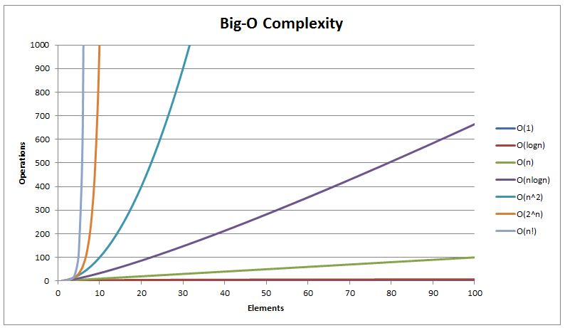
Here, the loop is not only carried out once, but once for an ‘n’ number of times. The runtime here is literally O(n) * O(n), or O(n^2). This is slower than both of the previous steps, meaning that this last one gets really, really slow as the input is larger.
Look at that line grow. Everything above the purple line is dangerously slow.
Take a look at this video by HackerRank to understand more about big O notation. This is a pretty basic overview. There are other cases to consider, like what if you have an ‘if’ statement where one condition takes constant time, and the other takes quadratic time? Here, you would still say the runtime of the algorithm is quadratic, or O(n^2). While doing big O notation, we are always looking for the worst-case runtime of the code. It doesn’t matter how fast it usually is, it’s about how slow it can be. Also, unlike I said earlier, even if for the official runtime, we consider the biggest value in the runtime as the number, the constants and multiples matter in real life. Just make sure you know that big O gives you a worst case scenario.
If you want a best case, look up ‘big omega notation‘, and if you want an average case, look up ‘big theta notation‘. Runtime just helps you get a feel for how long a task will take. Of course, if you work in CS, you’re job is to make sure that the runtime is as fast as possible, so work on improving it piece by piece. On a side note, don’t run with a USB stick in your hand. It looks suspicious. Next week, we’ll look at another concept, maybe sorting. Until then, good luck.
Today, we will be discussing some data structures. Now, what are data structures? Well, basically when you store any kind of object in your room, do you want it to be messy, or stuck in pile of god-knows-whatever objects and impossible to dig out until months later by accident? Or do you want it to (or hope it somehow will be) stored properly, where it is easily locatable? Hopefully, everyone picked the latter. Basically, a data structure is a tool that helps organize any incoming data in whatever order is required for that specific data.
Hopefully this isn’t you. I’m 99% sure this is a crime scene.
First, let’s look at a pretty well known data structure : Arrays. Arrays are a relatively common data structure, familiar to basically anyone with a highschool level understanding of CS. Basically, an array is like a whole group of numbers assigned to a variable. For example, if group of primitive integer variables are defined as :
g = 6
h = 7
y = 9
Instead you can define an array and say
j = {6,7,9}
A specific value in this array is marked with an “index”. Basically, each entry is labelled starting from 0. Here, j[0] would refer to the ‘6’. It gets a little confusing as you would expect j[3] to give ‘9’, but here since you start indices from 0, ‘9’ is actually j[2]. j[3] would be an error (rather an “exception“). To understand an array, just think of a table.
Not the most exciting table, but hey. Courtesy of Desmos.
Basically, if you try to put in j[0], the system would go to the first entry, move down however many values the number in the bracket specified, and return the corresponding entry. Arrays are pretty common, but it is reasonably complicated to remove or add elements to an array. Usually, arrays come in set sizes and stay that way.
Also, keep in mind that arrays can only store on dimensional data (basically just a line). If you need to store data for a whole grid, you need something better.
Presenting, two dimensional arrays!
Very creative name, I know.
Two dimensional arrays work pretty much the same way, except now you need to specify rows and columns, so j[0][3] refers to the value in row 0, column 3. Try not to think of it as an entirely new structure. A two-dimensional array is basically just an array of arrays, if that makes sense. Think of an array, but instead of each element j[n] referring to one specific number, it refers to a whole other array.
Let’s look at some other data structures. A linked list is a data structure that’s like a train. Each value in the list is a “node”, and all the nodes are joined so that each connects to the next one, and the next one and so on. Linked lists are good if you want to add and remove data quickly, you just have to make sure that the pointers going to the removed data are sorted out properly. Linked lists help you, well, link data. Suppose you have a bunch of nodes that were made at different times, so they are spaced out in the computer’s memory. With a linked list, you can join them all together and not have to worry about any data in between. A link list can either be circular, meaning that when you reach the end, it just points back to the start. Imagine a train going in an infinite circle (one of the most useless modes of transport ever created). It can also be a finite linked list, which ends whenever the node is a “null” or zero value. A doubly linked list is one that can go either front or back, so each value points both ahead and behind.
Just skip over the unnecessary one. Just like real life problem solving.
Let’s take a look at stacks, and queues. These are basically just different types of link lists. Queues are all “first-in-first-out”, basically whichever data arrives first is the one pushed out. Think of all the long queues at amusement parks. If you get there early, good on you! But if you don’t, you wait there politely until you can leave.
My god. Is the ride really worth it?
A stack is a last-in-first-out structure (all the people who ever had problems with recursion just shuddered). Imagine a pile of socks. Unfortunately, when you put your socks in a stack, the nice clean ones that you put on top end up getting used first, and the ones at the bottom never see the light of day again. Stacks basically work the same way. Any new data is “pushed” onto the stack, and the same data is the first thing “popped” off.
I have an intense fear of the word “Overflow” now.
Lastly, let us look at trees. A tree is basically a link list with a left and right side. Most people will know what a tree is, just picture all those awful family trees you had to make for school.
Ah yes, nature is so beautiful. Look at them bloom.
Each tree has “parent” and “child” nodes, which basically define if the current node points to anything else or not. The main node , or ‘8’ here, is known as the “root” node, which is odd considering the top of the tree isn’t really the roots, but sure. Trees come in allkinds, and there are even crazier kinds of trees that rotate to balance the number of nodes on each sides (nature in CS is weird).
Well, that’s pretty much it. Data structures provide a convenient way to store data so you don’t just lose it in a heap of random gibberish. Next week, we’ll look at some more in-depth things about, say, algorithms. Until then, good luck.
Considering how last time’s post was about how algorithms “learn”, let’s look at another way in which AI can advance – “Q-learning”. Q-Learning takes a different approach to teaching AI as compared to neural networks. Instead of just multiple rounds of trial and error wherein the AI learns what’s wrong, the AI is instead rewarded for doing good, and punished for doing bad. Try to imagine it like this :
Imagine the AI is a pig, that you want to teach how to stay in one place. In a neural network, first you would obtain a pig.
Pig obtained.
Then, you would wait to see what it did. Ideally, you would bring in more than just one pig.
They are coming.
Now, you would wait. If a pig does something good, you would then let that pig make lots and lots of little baby pigs, and those pigs would do the same. If the pig did something bad, you would get rid of it, and get another.
Good thing, too.
This tries to emulate the ideas of “natural selection”. Good behaved pigs go on to make others, and bad behaved pigs do not. Eventually, all the pigs then know what to do. However, this takes many versions of the pig, and makes a lot of excess bacon. In Q-learning, the pig would instead be given a reward every time it stayed for a long enough time, and punished if it did not. As a result, we get something a lot closer to how human children learn, with the principle of ‘Negative Reinforcement‘.
Good Piggy!
Like our pig friends, the AI would be put on an already created playing field where it wouldn’t know what to do. It would then slowly try to move around. If it did anything bad, it would get a punishment in the form of a low number, and if it did something good, then it would get a reward as a high number. The AI would keep trying out different things, and in the end, the AI would follow all the steps that give the best reward and thus learn to do whatever you want it to.
Q-Learning comes from the “Q-function”, or “quality function”. The AI would use this Q function for every task it does. The Q function is essentially modelled like this:
Q[s(state),a(action)]
Here, the function would consider the current state of the AI. It would then consider the action that the AI is about to take. The function would try to realize the immediate reward it would get for doing the current action, and all the future rewards that the current action would help it get later (the function isn’t “greedy”, it doesn’t try to just look at the immediate reward, it considers the future also). So, while actually working, the process is as follows :
π(s) = argmaxa(Q[s,a])
The ‘π(s)’ part represents the “policy” for state ‘s’, or the action we take in state ‘s’. The equation here tries to test all the possible actions we can take in state ‘s’, and then find the one that gives the maximum reward. A table is then made for all the possible rewards that the AI can get, and then the table is constantly updated as the AI performs more and more actions. The AI then does that over and over until there is a clear picture of what it should do. Finally, the AI can follow the path with the highest reward as listed in the table, and do whatever needs to be done.
For example, take a look at this explanation of the value functions and a simple approach to eating using Q-learning. Also, check out this video by Siraj Raval for a great explanation about how Q-learning works, and this video by Code Bullet again to see a cool car drive around a track with Q-learning. Well, that’s pretty much it for now. Next week, we’ll look at some other stuff with different AI algorithms. Until then, good luck.